Conflicting Employment Figures

The government's monthly survey of businesses indicates that payrolls experienced a net drop of 63,000 jobs during February. At the same time, numbers from the government's monthly survey of households indicated that the unemployment rate declined from 4.9% in January to 4.8% in February. How can the unemployment rate fall even as the economy sheds jobs? Understanding this paradox requires a closer look at the household survey numbers for the past two months.

* Numbers in thousands

The household survey indicates that the number of employed persons saw a net decline between January and February. The ranks of the employed thinned by about 255,000 people. Normally, the net drop in the number of employed people would cause the ranks of the unemployed to swell by a similar amount. The government considers a person unemployed if she lacks a job but has actively searched for one in the past four weeks. Yet, the pool of unemployed workers actually shrank by about 195,000 people between January and February. The change in the size of the labor force over the same period provides some clues as to why.

The number of people dropping out of the labor force in February exceeded the number of new entrants—on net about 450,000 people left the labor force. These people either left jobs with no intent of finding another or gave up on their employment searches altogether. If you want a job but you're so frustrated with past failures to find one that you stop looking, the government classifies you as a discouraged worker and no longer considers you to be part of the labor force.

All things being equal, February's employment drop of 255,000 should have increased the pool of unemployed workers from 7.58 million to 7.83 million. Things weren't equal though, as a number of people considered unemployed in January gave up on their job searches in February, contributing to the 450,000 person drop in the size of the labor force and causing the number of unemployed workers to come in at 7.38 million in February rather than 7.58 million. If we assume that all 450,000 people became discouraged workers in February, the drop in the ranks of the unemployed and, consequently, the labor force, reflects the inability of those out of work to find compatible job vacancies.

The unemployment rate is simply the ratio of unemployed people to the size of the labor force (unemployed / labor force). Since the ranks of the unemployed declined by 2.6% and the size of the labor force declined by only 0.3%, the fraction of the labor force considered unemployed declined from 4.9% in January (7,576 / 153,824) to 4.8% in February (7,381 / 153,374). In this peculiar case, the small drop in the unemployment rate reflects economic weakness rather than economic strength.

Discussion Questions

1. Here's what the employment numbers for February would have looked liked if the 450,000 people who left the labor force had remained in the labor force as jobless workers actively searching for employment (unemployed people):


* Numbers in thousands

Under these conditions, what would the unemployment rate have been for the month of February 2008?

2. You can find the Bureau of Labor Statistic's (BLS) news release for February 2008 here. The national unemployment rate is at best a rough gauge of joblessness in the United States. The February numbers illustrate how the unemployment rate can paint a misleading picture of labor market strength. A fuller understanding of labor market issues requires a closer look at employment figures. How do the unemployment rates for specific age and racial groups differ from the national rate?

3. According to the BLS, who are the people who “work part time for economic reasons”? What has happened to their numbers over the past year? Does the unemployment rate capture changes in the number of folks who work part time for economic reasons?

4. Our assumption that all 450,000 people who left the labor force in February became discouraged workers is unrealistic. (Indeed, the BLS only counted a total of 396,000 discouraged workers in February.) Who, according to the BLS news release, is considered a “marginally attached worker”? Are all marginally attached workers also discouraged workers?

5. An unemployment rate of just below 5% is still relatively low by historical standards. Nonetheless, tepid employment reports in January and February darken the U.S. economic outlook when considered along side reports of weak output growth and continuing turmoil in housing and financial markets. Keeping in mind that the Fed's recent rate cuts and the government's tax rebates will begin to impact the economy in May and June, what type of economic performance do you expect in the United States for 2008?

The Phillips Curve and the Federal Reserve

The Phillips Curve is a concept often covered in introductory macroeconomics. However, in some economic and political circles, the concept is considered outdated and useless. Some economists and commentators, such as Lawrence Kudlow, might go as far as to say that the Phillips Curve is dead. Why does the Phillips Curve command such controversy? Is it as irrelevant as some economists claim?

The traditional Phillips Curve is the trade-off between the inflation rate and the unemployment rate. Many economists in the 1960s thought that the Federal Reserve or Congress could permanently lower the unemployment rate by increasing the inflation rate. The trouble is, the traditional Phillips Curve violates one of the central tenets of economics: the classical dichotomy. According to the classical dichotomy, nominal variables do not affect real variables. Consider a simple example:

I hold a bag of apples that weighs 5 pounds. The weight (i.e., the force exerted on my arm) is a real variable and the unit of measurement (i.e., pounds) is a nominal variable. Suppose the U.S. government passes a new law that says all measurements must conform to the metric system. Now the same bag of apples weighs 2.27 kilograms. Notice that the nominal variable (how the weight is measured) has absolutely no effect on the real variable (the force exerted on my arm).

The traditional Phillips Curve is in direct contradiction of the classical dichotomy. The Phillips Curve implied that the government could effectively reduce the unemployment rate (a real variable) by changing how fast overall prices are growing in the economy (a nominal variable). Though the traditional Phillips Curve held up well in the 1960s, the 1970s would usher in the downfall of the traditional Phillips Curve.

In the 1970s, the trade-off between the unemployment rate and the inflation rate seemed to fall apart. The United States experienced soaring overall prices and rising unemployment. In other words, there appeared to be an upward-sloping relationship between the inflation rate and unemployment rate. Due to this fact, many economists declared the Phillips Curve to be dead.

Due to the abrupt change in the correlation between inflation and unemployment, several theories were proposed as alternatives to the Phillips Curve. These theories include the Real Business Cycle (RBC), Rational Expectations, and Monetarism. Often times these theories are called “New Classical” economics because they promote the classical dichotomy.

Under heavy pressure from competing theories and empirical evidence, a new school of thought known as “New Keynesian” economics sought microeconomic foundations for the Phillips Curve. Edmund Phelps, the Nobel Laureate in 2006, augmented the traditional Phillips Curve by adding the critical role of expectations. Under the expectations-augmented Phillips Curve model, a trade-off between inflation and unemployment does exist but only in the short run. According to the model, inflation expectations adjust to return the economy to its natural rate of unemployment (i.e., an unemployment rate consistent with non-accelerating inflation). George Akerlof, the Nobel Laureate in 2001, provided behavioral explanations for the trade-off. Subsequent works by economists, such as David Romer and Greg Mankiw, provided additional microeconomic foundations for a short-run trade-off.

Through all the intellectual turmoil, most economists agree on the following:

1. There is a short-run trade-off between the inflation rate and the unemployment rate.
2. In the long run, the inflation rate adjusts to restore the natural rate of unemployment. Hence, policy makers cannot permanently push unemployment below its natural rate by permanently increasing the inflation rate.

How well does the modern Phillips Curve describe the real world, and do practitioners actually use the modern Phillips Curve? James Stock and Mark Watson, authors of a famous introductory econometrics textbook and well-respected econometricians, empirically showed that the modern Phillips Curve bested all other alternatives in terms of forecasting inflation. Ben Bernanke, chairperson of the Federal Reserve, professed publicly here and here on the importance of the modern Phillips Curve in the Fed's inflation forecasts, which ultimately influence monetary policy.

The Phillips Curve has changed over the past 40 years, but it is very much alive as a reference for monetary policymakers.

Discussion Questions:

1. Go to the Bureau of Labor Statistics web site and pull data on the national unemployment rate and the CPI inflation rate. For your convenience, I have included the spreadsheet here. Does there appear to be a trade-off between inflation and unemployment between January 2001 and December 2001?

2. Does there appear to be a trade-off between January 1997 and October 2007?

3. Why do you think an increase in the inflation rate decreases the unemployment rate in the short run? Why do you think a decrease in the unemployment rate increases the inflation rate in the short run?

Loss Aversion and the Housing Market

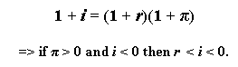
For many people, the pain of losing $500 outweighs the pleasure of gaining $500. As Austan Goolsbee points out in a recent New York Times column, this aversion to loss is especially acute when it comes to selling real estate. People are stubborn about selling a house for less than they paid for it. If selling at prevailing market prices means accepting a significant loss, some people refuse to sell at all, or else base pricing decisions not on what they would willingly pay to buy a similar house today, but rather on what they paid for the house when they bought it. As a result, sellers who bought houses during the peak of the housing boom will list their properties for a higher price than nearly identical homes purchased earlier on at lower prices. At worst, the strong reluctance to sell at a loss leads to a prolonged freeze in the housing market, with many homes listed for sale at prices that buyers will not pay. Since people who sell a house often go on to purchase another, loss aversion can contribute to weaker housing demand and prolong the housing slump.

The housing correction in the U.S. continues to reduce house prices in many regional markets. The correction raises the risk of a downturn in the U.S. economy. As house prices decline (other things being equal), household wealth declines, and consumption expenditures decrease. The shock to consumption spending may contribute to slower growth or even a recession. As Goolsbee points out, loss aversion in the housing market adds to the gloomy outlook for the broader economy. The reduction in housing-market transactions affects the consumption of durable goods and increases the costs associated with switching jobs. Read Goolsbee's column to find out more.

Discussion Questions

1. According to the article, what fraction of home buyers are moving within a metropolitan area? How will seller reluctance to lower prices during a housing slump affect the number of future buyers in a local housing market?

2. Suppose a beet farmer arrives at the farmers' market only to discover that other beet farmers are selling identical beets for less than he had intended to sell his own beets. He is likely to succumb to competitive forces and sell his beets at the prevailing price. Why are house sellers, unlike beet farmers, unwilling to lower their prices? Does it have to do with characteristics of the sellers or characteristics of the markets?

3. What are durable goods? Why would this type of housing-market freeze impact sales of durable goods? Why do you think the ups and downs of durable-goods sales are closely aligned with the ups and downs of the business cycle?

4. Frictional unemployment refers to the relatively short spells of unemployment associated with finding and transitioning to a new job. For example, a recent college graduate searching for her first job or a banker transitioning between jobs in different areas will be frictionally unemployed until they start at their new positions. How might a prolonged housing freeze increase frictional unemployment? To what extent might a housing freeze cause people to stay in jobs they would otherwise leave?

Oil Shock, Part II: The Macroeconomic View

Microeconomists examine how the BP oil field shutdown affects oil prices, the behavior of automobile drivers, and profitability of particular industries. Oil Shock, Part I showed that the oil field shutdown raises the price of oil which reduces the profitability of many firms.

Macroeconomists, on the other hand, examine the economy-wide effects such as how a sharp rise in oil prices affects inflation, output, and unemployment. Suppose that the BP oil field shutdown causes the inflation rate to increase from Inflation Rate 1 to Inflation Rate 2 because firms try to pass on some of the higher input prices to higher output prices. In order to simplify the analysis, assume that full-employment output is constant at FE Output. Full-employment output, or potential output, is the amount of output that the economy produces when all the resources in the economy are efficiently utilized.

If the BP oil field shutdown increases the inflation rate, then the Fed will pursue a tight (anti-inflation) monetary policy which raises interest rates. Higher interest rates would reduce consumption and investment, causing output to fall. An output gap opens up as actual output falls below full-employment output in the short run. In the long run, the output gap will cause the inflation rate to fall back to its initial state. As the inflation rate falls in the long run, the Fed will pursue loose monetary policy and return the economy back to full employment.

A fall in output usually leads to an increase in the unemployment rate as firms cut back on production of goods and services and lay-off workers.

If the BP oil field shutdown leads to an inflation shock, then interest rates will rise, output will fall, and unemployment will increase in the short run.

However, inflation's tyranny does not end there. A higher inflation rate also destroys wealth in terms of stocks and bonds. An increase in the interest rate also reduces the price of stocks and bonds (archived entry: Why Does Bernanke's Small Talk Move Markets?)

1. Financial markets are very sensitive to inflation data. Suppose the Bureau of Labor Statistics reports that the inflation rate increased from 2% to 4%. Why would stock and bond prices fall as soon as the report is released, but before the Fed actually changes any interest rates?

2. The Fed, in its last FOMC meeting on August 8, 2006, kept the federal funds rate unchanged at 5.25%. Could this mean that the Fed does not consider the BP oil field shutdown an inflation shock?

3. Inflation expectations matter. The Fed's inflation-fighting credibility has been strong since Paul Volcker (the Federal Reserve Chairman from 1979 to 1987). Suppose consumers and producers always expect the Fed to return the economy to a target inflation rate--would higher oil prices require the Fed to raise interest rates (or raise them by as much)?

Bringing the French Unemployment Picture Into Focus

News reports consistently cite the high unemployment rate for young people in France. According to the OECD, in 2002 the unemployment rate for French 20- to- 24-year-olds was 15.5%. This is higher than many other industrialized countries--for example, the same figure for Canada was just 7.2%, less than half of the French statistic.

However, while the difference in the unemployment rate between two adjacent years in the same country can tell you a lot about the state of the economy, the difference in unemployment rates between two countries is harder to interpret because so many factors can differ. To make a meaningful comparison of the labor market in two countries, it helps to look at other variables besides the unemployment rate. For example, the same OECD report also shows that the fraction of all 20- to- 24-year-olds who were unemployed was 8.4% in France, compared to 5.7% in Canada--higher to be sure, but by much less.

How can these two measures of joblessness paint such different pictures? Might it be that labor market conditions in France are not as bad as the unemployment rate suggests? Recall that the unemployment rate is the fraction of the labor force that is unemployed, not the fraction of the population. The unemployment rate is higher in France because a smaller fraction of 20- to- 24-year-olds are in the labor force there. The labor force participation rate for this age group is 54% in France and 79% in Canada.

These rates mean that for every 1000 20 -to- 24-year-olds in France, 540 say they want to work and 84 of them are unemployed, which leads to an unemployment rate of 84/540 or about 15%. For every 1000 20- to- 24-year-olds in Canada, 790 are in the labor force and 57 of them are unemployed, which leads to an unemployment rate of 57/790 or about 7%.

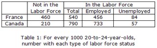
Yet other statistics show more clearly that the labor market opportunities for some young people in France are in fact much worse than in Canada. One useful measure is the duration of unemployment. For each 1000 young people in France, take the 84 who are in the labor force and unemployed. Of these, 34 have been unemployed for more than 6 months. Of the corresponding 57 people who are unemployed in Canada, only 5 have been unemployed for this long. (See Table 2, below.) This tells you that on average, spells of unemployment last much longer in France.

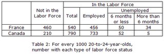
So the two major differences between France and Canada are (1) France has a lower labor force participation rate, and (2) long-term unemployment is much more prevalent in France. There are several explanations for these differences. A recent article in the Financial Times suggested that the main reason for the lower labor force participation rate may be that more twenty-somethings in France attend university. In fact, this can account for only a small part of the difference. The fraction of 20- to- 24-year-olds in education is only five percentage points higher in France--44% compared with 39% in Canada. Most of the 25 percentage point difference in labor force participation rates must therefore arise for some other reason.

A more troubling explanation for both differences is that many young people in France stay out of the labor force because they are discouraged--that is, they have been unemployed for so long that they do not feel that they can find a job, so they stop looking. Or they never bother to look. How many students would try to find a summer job knowing that it could take more than a summer’s worth of searching to find one? If many of the people who are out of the labor force would actually like to work but are so discouraged that they don’t even try, the human cost of France’s labor market rigidities may be even higher than its unemployment rate suggests.

1. Students across France have been protesting a new law that would make it easier for French employers to fire young workers. How might the passage of such a law affect the unemployment rate and the labor force participation rate? Why?

2. France has an unusually high minimum wage. Consider two groups: young people who have completed high school and drop outs who haven’t. Which group would you expect to have more unemployment because of the minimum wage? Would you expect this unemployment to be short-term or long-term?

3. Suppose the poor labor market for French youth encourages French students to stay in school longer than they would otherwise choose to, earning postgraduate degrees. What long-term effect would this have on the French economy?

Paul Romer is currently the STANCO 25 Professor of Economics in the Graduate School of Business at Stanford University and the founder of Aplia.

Youth Unemployment in France

Dominique de Villepin, France's prime minister, wants to loosen job protection rights for young workers. A recent Financial Times article (de Villepin labour reforms) highlights de Villepin's labor proposal. Existing French labor laws make it difficult and expensive for French firms to fire workers. The laws intend to prevent companies from dismissing employees on a whim. But job protection rights have some unintended consequences as well.

To analyze the effects of the laws, imagine yourself as a French business owner. Suppose a young, inexperienced worker applies for a position with your firm. There's a 50 percent chance she will work hard and a 50 percent chance she will slack off. You might be less willing to take a chance on this inexperienced worker if you face high dismissal costs in the event that she's a slacker. In short, French laws designed to protect workers actually create a disincentive for businesses to hire young, inexperienced workers in the first place. Some argue that this accounts for the sky-high youth unemployment rate in France, which currently stands at 23%--and even higher among immigrant populations.

De Villepin's reform would allow companies to hire workers ages 26 and under on a two-year trial basis. If a young worker excels during the two-year trial, she gets a full-time contract and all of the job protection rights that come with it. But if she doesn't, the employer could let her go at no cost. De Villepin argues that these looser firing restrictions would encourage firms to hire more young workers, driving down the youth unemployment rate.

De Villepin is not the first to propose such reforms. Each time officials proposed youth labor reforms in the past, massive labor union and student protests derailed the legislation--de Villepin can expect more of the same.

1. In addition to job protection measures, France offers comparatively generous unemployment insurance payments and high minimum wages. How do these policies affect the demand for inexperienced youth labor?

2. Would you classify the unemployment created by government legislation such as the minimum wage or firing restrictions as structural, frictional, or cyclical?

3. French officials defend job protection measures, arguing that job security makes workers happier, and therefore more productive. How might job protection measures affect worker productivity?

4. If you were a student in France, would you join the protests or endorse de Villepin?

Topics: Labor market, Unemployment, Structural reforms